Example: Fitting a dimer binding curve with the SCME Code¶

Note

In this example we will learn how to find the optimal SCME parameters to reproduce the binding energies of an H2O dimer.

Obtaining data¶

The first step is, of course, to obtain all the reference configurations as well as the reference energies.

Note

Example data for dimer binding energies, computed with the PBE functional, can be found here. To follow this little tutorial, download all of these files and save them in a folder ./data.

Generally, it is a good idea to store the paths to the reference configurations, reference energies and some tags in a file somewhere on your computer. In the example data above, this file is called energies.csv. It has three columns (if you ignore the index): file, reference_energy and tag.

We are very lucky since the process_csv() function provides a utility to parse exactly this information from a CSV file:

from chemfit.data_utils import process_csv
paths, tags, energies = process_csv("./data/energies.csv")

Of course, you are free to obtain the list of paths, tags and energies in any other way as well.

Parameters¶

This section describes how to specify the parameterization of the SCME.

Default Parameters¶

First, we have to decide the default parameters of the SCME to be used, these are the parameters passed into the calculator upon initial construction.

The default parameters are supplied as a simple nested dictionary.

Not all of the default parameters will be changed during the optimization, but even if they remain constant they need to have a value … specifying these constant values is the purpose of the default_params dictionary.

Here is an example of how the default params can be constructed:

from ase.units import Bohr

default_params = {
    "dispersion": {
        "td": 4.7,
        "rc": 8.0 / Bohr,
        "C6": 46.4430e0,
        "C8": 1141.7000e0,
        "C10": 33441.0000e0,
    },
    "repulsion": {
        "Ar_OO": 299.5695377280358,
        "Br_OO": -0.14632711560656822,
        "Cr_OO": -2.0071714442805715,
        "r_Br": 5.867230272424719,
        "rc": 7.5 / Bohr,
    },
    "electrostatic": {
        "te": 1.2 / Bohr,
        "rc": 9.0 / Bohr,
        "NC": [1, 2, 1],
        "scf_convcrit": 1e-8,
        "max_iter_scf": 500,
    },
    "dms": True,
    "qms": True,
}

Warning

Every parameter, which is not specified in the default parameters, implicitly relies on the defaults set within the SCME code. It might be a good idea to review these defaults and to not rely on them as they might be subject to change.

Initial Parameters¶

We should now also decide which of the parameters we want to optimize in order to approach the reference energies. This is done by specifying a dictionary of initial parameters

initial_params = {
    "electrostatic": {"te": 2.0},
    "dispersion": {
        "td": 4.7,
        "C6": 46.4430e0,
        "C8": 1141.7000e0,
        "C10": 33441.0000e0,
    },
}

Note

Every (key,value) pair in the initial_params dictionary is subject to optimization by the Fitter starting from the initial value given in the dict.

Note

If a key is found both in the default_params and the initial_params, the initial_params just overwrite it upon application of the parameters.

Using monomer expansions¶

Lastly, we should decide if we want to use monomer expansions in the style of the generalized SCME code. These are supplied in the form of a path to an HDF5 file (path_to_scme_expansions argument) and a corresponding key to the expansion dataset in this file (parametrization_key argument).

If any of these are None, the generalized SCME will not be used.

Instantiating the factory functors¶

While it is completely possible to supply your own factory functions, we will use the predefined ones from the scme_factories module:

from chemfit.scme_factories import SCMECalculatorFactory, SCMEParameterApplier

calc_factory = SCMECalculatorFactory(
                    default_scme_params=default_params,
                    path_to_scme_expansions=None, # we do not use the generalized SCME in this example
                    parametrization_key=None
                )

param_applier = SCMEParameterApplier()

Instantiating the objective function¶

For each configuration, we now instantiate a QuantityComputerObjectiveFunction() from a SinglePointASEComputer() and combine them in a CombinedObjectiveFunction.

As the loss function we use

\[\text{L} = \sum_i \left( \frac{E_i - E^\text{ref}_i}{n_\text{atoms}} \right)^2.\]

from chemfit.abstract_objective_function import QuantityComputerObjectiveFunction
from chemfit.ase_objective_function import SinglePointASEComputer, PathAtomsFactory
from chemfit.combined_objective_function import CombinedObjectiveFunction

def make_energy_term(path, tag, e_ref):

    comp = SinglePointASEComputer(
        calc_factory=calc_factory,
        param_applier=param_applier,
        atoms_factory=PathAtomsFactory(path),
        tag=tag,
    )

    # Example normalization by n_atoms**2 (as in tests)
    return QuantityComputerObjectiveFunction(
        loss_function=lambda q, e=e_ref: (q["energy"] - e) ** 2 / (q["n_atoms"] ** 2),
        quantity_computer=comp,
    )

terms = [make_energy_term(p, t, e) for p, t, e in zip(paths, tags, energies)]
ob = CombinedObjectiveFunction(terms)

Performing the fit¶

Pass the objective function to an instance of the Fitter class and write some outputs

from chemfit.utils import dump_dict_to_file
from chemfit.fitter import Fitter

fitter = Fitter(
    objective_function = ob,
    initial_params = initial_params
)

# All keyword arguments get forwarded to scipy.minimize
optimal_params = fitter.fit_scipy(
    tol=1e-4, options=dict(maxiter=50)
)

# We can print the optimal parameters and some information about the fit
print(f"{optimal_params = }")
print(f"{fitter.info = }")

# Optional: save the parameters to a JSON file
dump_dict_to_file("output_dimer_binding/optimal_params.json", optimal_params)

Getting per-term data¶

After the fit we can gather the meta data and thus evaluate per-term contributions.

Note

Since the meta data capture data for the last evaluation of params it is good practice to execute an evaluation of the objective function for the optimal parameters. The reason for this is that it is not guaranteed that the last evaluated parameter set is the optimal one.

ob(optimal_params)

# Gather the meta data (a list of dict)
meta_data = ob.gather_meta_data()

# Use a list comprehension to retrieve the fitted energies
energy_fitted = [md["computer"]["last"]["energy"] for md in meta_data]

Expected results¶

If the fitted energies are plotted against the reference it should look something like this

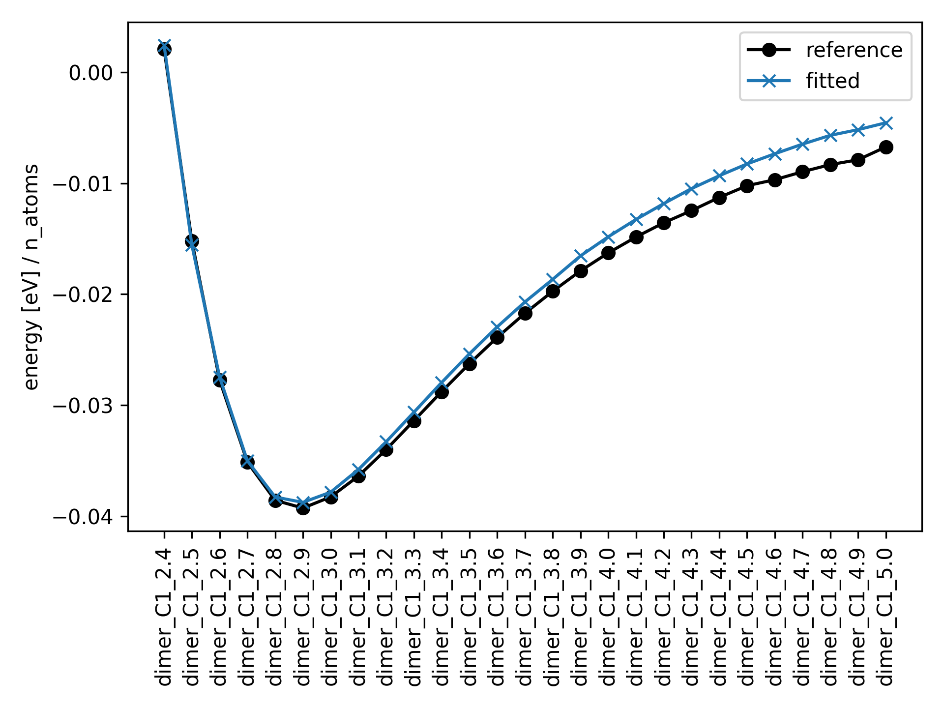
The optimal parameters should be saved as a json file called output_dimer_binding/optimal_params.json:

{
    "td": 1.7307507548872705,
    "te": 3.3319409063023553,
    "C6": 334.4715463605395,
    "C8": 1146.9930705691029,
    "C10": 33441.07679944017
}

Lastly, there should be a CSV file output_dimer_binding/energies.csv containing information about each reference configuration in each row.